
 500 feet to go – Don’t fall down now!
Many of you who read my earlier blog entry, 26.2: The Engineering of Marathon Racing, are aware that I was training for the Chevron Houston Marathon. To those who wondered how I fared, I am proud to say that on January 17 I completed my first (and last!) marathon with flying colors. If anyone is looking for a challenge in life, I cannot recommend a more rewarding experience than taking on your first marathon.

26.2 miles is a long time to be out on the road, a long time with nothing to do – besides putting one foot in front of the other 42,000 times – but people watch (after all there were 13,500 other equally crazy people huffing and puffing in front of me). People watching is the easy part, since marathon runners tend to skew toward the physically fit and the attractive, with nearly half of the runners being women. As I watched lady after lady run past me over the course of several hours, I gradually realized that a marathon could provide a perfect teachable moment for any engineer interested in better understanding structural dynamics.
I’ve written articles on structural dynamics before, for example: This Joist is Jumpin’: the Structural Dynamics of Dance. But some readers wnat more: “I sort of get it, but can you go over it again?” So 20 miles into the race, when other runners were hitting “the wall”, I started formulating in my mind a new way of illustrating the principles of structural dynamics. Here on all sides of me were real life examples of Dynamic Load Factor (DLF, or the ratio of dynamic response to static response) demonstrating the three types of dynamic response: Flexible (a dynamic response less than the static response under the same load), Resonant (a dynamic response greater than the static response), and Rigid (a dynamic response about the same as the static response).
The women runners, with their constant strides, represent nearly perfect harmonic load functions. The dynamic response? Well it is hard not to notice the resulting bounce of a certain part of their bodies – bounce that varies from individual to individual – but which can still be easily classified as falling within one of the three response types listed above.
Yes, guys, you all know what I’m talking about: their hairstyles. After watching 6700 women runners pass by, it’s clear that some of the hairstyles do not bounce up and down as much as the head does (by definition a Flexible Response), some hairstyles move much more than the head does (Resonant Response), while still other hairstyles follow the movement of the head nearly exactly (Rigid Response). The fun part for an engineer is deriving the dynamic formulas that explain this phenomenon, in between chugging Gatorade and downing Power Bars.
First, let’s review the theory. Structural dynamics says that the DLF, for a harmonic load (a load that is applied with a uniform time cycle, such as a runner’s cadence), is dependent on one thing: the ratio of the Forcing Frequency (ff) of the applied load to the Natural Frequency (fn) of the responding system (well, there is one more thing, damping, but we will ignore that for now).
As we see from the plot below, when the Forcing Frequency is less than the Natural Frequency (ratio approaches 0), the dynamic response is Rigid, and the response is approximately equal to the input. However, when the Forcing Frequency exceeds the Natural Frequency (ratio approaches Ꝏ), the dynamic response is Flexible, which means that the response is less than the input. And finally, when the Forcing Frequency and Natural Frequency are close to each other (ratio approaches 1.0), the response is Resonant, which means that the hair bounces all over the place.
 So how can this explain runners’ hair? For examples we turn to a wonderful video put together by TTBikeFit LLC, analyzing the performance of the top women in the 2013 Boston Marathon. A dedicated distance runner is welcome to watch the full 18 minutes, an engineer needs only watch the following few second clips.
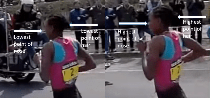
First, we have Kenya’s Rita Jeptoo, running at a cadence of 95 paces per minute (a harmonic load with a frequency of 1.6 Hz):
What can do we notice about Rita’s hair in this clip? Basically her hair does bounce up and down as she runs, but not as much as her head (the load transmitter) does. In order to see this better, I have excerpted stills from the video which show the lowest and highest vertical positions of the hair and nose (a good surrogate for head position). Note that the timing of the lowest hair position does not coincide with the timing of the lowest nose point position — dynamic response is often out of phase with dynamic loading.

 Go Rita Go!
Scaling the points on the photo, it appears that Rita’s hair bounces up and down through a range of 1.25 inches, while her nose moves up and down a total of 1.75 inches. If the head motion had been applied statically, the displacement of the hair would have been 1.75 inches, whereas the actual dynamic response was only 1.25 inches. So the DLF of Rita’s hair is:
DLF = 1.25/1.75 = 0.71
Since this DLF is less than 1.0, it indicates that the hair does not fully respond to the applied dynamic load (the head bouncing up and down) – a reaction defined as a “Flexible Response”.
Next let’s take a look at the second place runner, Ethiopia’s Meseret Debele. Her hair is much tighter to her head, and seems to rise and fall to exactly the same extent:
Extracting stills from this video clip confirms this (note that we only need to extract one set of stills from clip, since the high and low points of the hair and the nose coincide):
 Come on Meseret, you can do it!
The difference between the highs and lows here are almost identical – scaling, I get about 2.2 inch bounce in the hair vs. 2.1 inch bounce in the nose. So in this case the DLF is:
DLF = 2.2/2.1 = 1.05
Since this DLF is approximately 1.0 (at least within the margin of error of my measurements), it indicates that the hair fully responds to the applied dynamic load. This type of response is called as a “Rigid Response”.
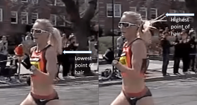
Finally, let’s take look at the USA’s Shalane Flanagan, in fourth place. Her hair flies all over the place, obviously moving up and down much more than her head does.
Extracting stills from the clips as before:
 Don’t look back, Shalane, something might be gaining on you!
Scaling these points gets a hair displacement equal to 13 inches vs. a nose displacement of 3 inches, or a DLF of:
DLF = 13.0/3 = 4.33
Since this DLF is greater than 1.0, it confirms what our eyes tell us – that the dynamic response of the hair exceeds the applied input load. This type of response is called a “Resonant Response”.
Why do these different hairstyles have different dynamic responses? As explained by the theory above, the response is determined by the ratio of Forcing Frequency to Natural Frequency. The Forcing Frequencies (running cadences) of these three runners are nearly the same — 95, 101, and 90 steps per minute — so the difference must lie instead in the Natural Frequencies of the individual hairstyles.
Structural dynamics theory tells us that Natural Frequency depends on a system’s stiffness K and mass M:
Natural Freq (Hz) = (√ K / M) / (2π)
So let’s examine the structural makeup of the hairstyles.
Rita’s hair is rolled into a ball of about 0.075 m diameter, which is suspended approximately 0.065 m from the tie point on her head, by a cylindrical hair braid of about 0.025 m diameter. This can be approximated as a cantilever with a mass on the end:
 Engineering blueprints of Rita’s hairstyle
The natural frequency calculation for this configuration is:
Natural Freq (Hz) = (√ 3 E I / M L3) / (2π)
The volume of the 0.075 m sphere is 2.2E-4 m3. Density of hair is around 1330 kg/m3 (reference) — assuming the hair is packed at a 3:1 air-to-hair ratio, this indicates a mass of 2.2E-4 * 1330 / 4 = 0.073 kg.
The cantilever part is actually many individual cantilevers (individual hair strands) acting independently. Typical hair density is 3,400,000 strands per square meter (reference), so the braid contains around π 0.01252 * 3.4E6 = 1650 hairs. So each hair supports 1/1650 of the mass (0.073 kg/1650). The diameter of a typical hair is 75E-6 m (reference), so each hair’s moment of inertia I = π 75E-64 / 64 = 1.55E-18 m4. The modulus of elasticity E of hair is 7.0E9 N/m2 (reference). So the Natural Frequency of Rita’s hairstyle can be estimated as:
Natural Freq = (√ 3 * 7E9 * 1.55E-18 / ((0.073/1650) * 0.0653) / (2π) = 0.26 Hz
So the Natural Frequency of Rita’s hairstyle (0.26 Hz) is much less than the Forcing Frequency of her running cadence (1.6 Hz), validating our observance of a DLF less than 1.0. This explains the Flexible Response – hair bouncing less than her head.
Still with me? Let’s check out Meseret’s hairstyle. Looking at the photos, it can probably best be approximated as a short, thick cylindrical cantilever sticking straight out the back of her head, with a length L of approximately 75 mm and a diameter of 100 mm.
 Structural model of Meseret’s hair
The fundamental Natural Frequency of a uniform cantilever is calculated as:
Natural Freq (Hz) = 1.8752 √ (E I / (ρ A L4))
Once again evaluating the hairs as independently acting uniform cantilevers (but this time without a concentrated end mass):
Natural Freq = 1.8752 √(7.0E9 * 1.55E-18/(1330 * π 3.75E-62 * 0.0754)) = 268 Hz
The Natural Frequency of Meseret’s hairstyle far exceeds the Forcing Frequency of her pace, so it is not surprising that the DLF is nearly 1.0, confirming our observation of a Rigid Response – hair closely following the head motion. Once again engineering explains reality!
At this point I’m sure you all have caught on. So I leave it to you to check my math, as well as confirm that the Natural Frequency of Shalane’s hairstyle predicts a Resonant Response. It’s time for me to head out on a training – and people watching — run!
Having a bad hair day? You can always fix things structurally, using CloudCalc, the scalable, collaborative, cloud-based structural engineering software. www.cloudcalc.com – Structural Analysis in the Cloud.
By Tom Van Laan
Copyright © CloudCalc, Inc. 2016
